When is a triangle not a triangle?
(when it's compressed)
Welcome to this 6th in the series of blog posts examining the task of creating a Blender Addon to assist with our Second Life Mesh creation workflows.In the last post, we discovered that all was not quite as it seems in the mesh streaming calculation. Our carefully recreated algorithm repeats all the steps that the published documentation discusses and yet the results did not match. We further learned that this was most likely down to the "estimation" process.
So what is the problem here?
The clue is in the name, "Mesh Streaming Cost" it is intended to "charge" based on the cost of streaming the model; so what does that mean? In real terms it means that they are not looking at the difficulty of rendering an object directly, they are looking at the amount of data that has to be sent across the network and processed by the client. When we export models for use in Second Life we typically use Collada format. Collada is a sprawling storage format that uses a textual XML representation of the data it is very poorly suited to streaming across the internet. This problem is addressed by the use of an internal format better suited to streaming and to the way that a virtual world like Second Life works.
What does the internal format look like?
We can take a look at another of the "hidden in plain sight" wiki pages for some guidance.
The Mesh Asset Format page is a little old, having last been updated in 2013 but it should not have fundamentally changed since then. Additions to SL such as normal and specular maps are not implemented as part of the mesh asset and thus have no effect. It may need a revision in parts once Bento is released.
The page (as with many of the wiki pages nowadays) has broken image links. There is a very useful diagram by Drongle McMahon that tells us a lot about the Mesh Asset Format in visual terms.

In my analysis of the mesh streaming format, it became clear that while Drongle's visualisation is extremely useful it lacks implementation specific details. In order to address this, I looked at both the client source code but also the generated SLM data file for a sample mesh and ended up writing a decoder based upon some of the older tools in the existing viewer source code.
{ 'instance':
[ # An array of mesh units
{ 'label': 'Child_0', # The name of the object
'material':
[ # An array of material definitions
{ 'binding': 'equatorialringside-material',
'diffuse': { 'color': [ 0.6399999856948853,
0.6399999856948853,
0.6399999856948853,
1.0],
'filename': '',
'label': ''},
'fullbright': False
}
]
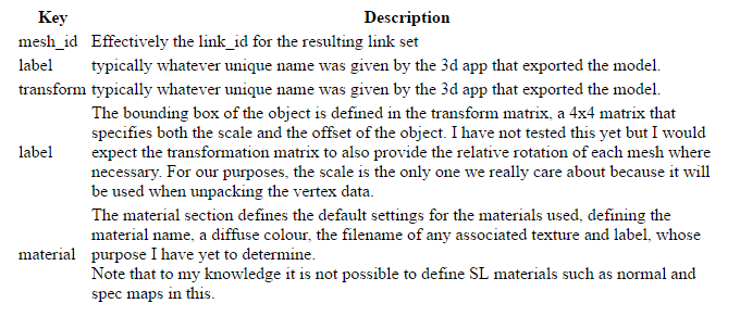
'mesh_id': 0, # A mesh ID, this is effectively the link_id of the resulting linkset
'transform': [ 10.5, 0.0, 0.0, 0.0,
0.0, 10.455207824707031, 0.0, 0.0,
0.0, 0.0, 5.228701114654541, 0.0,
0.0, 0.0, 2.3643505573272705, 1.0]
}
],
'mesh':
[ # An array of mesh definitions (one per mesh_id)
{ # A definition block
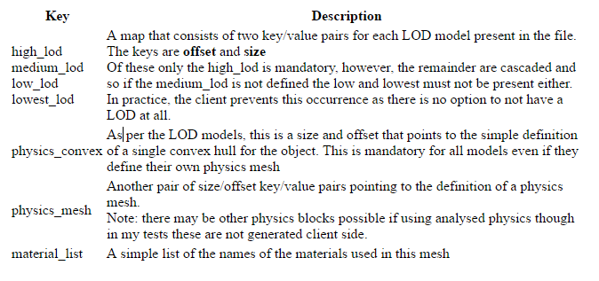
'high_lod': {'offset': 6071, 'size': 21301},
'low_lod': {'offset': 2106, 'size': 1833},
'lowest_lod': {'offset': 273, 'size': 1833},
'material_list':
[ # array of materials used
'equatorialringside-material',
'equatorialringsurface-material',
'glassinner-material',
'glassouter-material',
'strutsinnersides-material',
'strutsinnersurface-material',
'strutsoutersides-material',
'strutsoutersurface-material'
],
'medium_lod': {'offset': 3939, 'size': 2132},
'physics_convex': {'offset': 0, 'size': 273}
<compressed data="">
     # LENGTH=SUM of all the size parameters in the LOD and Physics blocks
    }
   ],
  'name': 'Observatory Dome', # name of the given link set
  'version': 3  # translates to V0.003
}
All of this is an LLSD, a Linden Lab structure used throughout the SL protocol, effectively an associative array or map of data items that is typically serialised as XML or binary. The header portion contains version information, and an asset name, it can also have the creators UUID and the upload date (if it came from the server) .
We also see two other top level markers, 'instance' and 'mesh', this is the stuff we really care about.
Instance
'Instance' is an array of mesh units that form part of the link set. Often when people work with mesh they use a single mesh unit but you can upload multipart constructs that appear inworld as a link set.Each instance structure contains a set of further definitions.
Mesh
The final entry in the header is the mesh array. Like the instance array before it the mesh array has one entry for each mesh unit and as far as I am able to tell it must be in Mesh_id order.The mesh structure in the array is another LLSD with the following fields:-
At the end of each Mesh is the compressed data that is represented by the bulk of Drongle's diagram and it is for this that we have been waiting for this is why our naive triangle counting solution is giving us the wrong answer.
Compressed mesh data
At the end of each Mesh block is an area of compressed data. Space for this is allocated by the SLM "mesh" entry whose length includes the compressed data even though it is not strictly part of the LLSD.
Once again we need to look at both Drongle's excellent roadmap and the viewer source code to work out precisely what is going on.
As you will recall the Mesh section defined a series of size and offset values, one pair per stored model. In my examples, the physics_convex is always the first model and thus has offset 0.
physics_convex
{ 'BoundingVerts': 'ÿÿÿ\x7f\x00\x00\x81Ú\x81Úa\x18þ\x7fæyþÿÿ\x7f\x00\x00\x
8}%\x81Úa\x18\x00\x00ÿ\x7fa\x18}%}%a\x18ÿ\x7fÿÿa\x181Ö\x16\x86\x97¸Ì)\x17\
                   '¯nÈ\x97¸\x00\x00ÿ\x7f\x00\x00\x9eO\x9aÇ\x94¸Äµ\x92í2\x
                   ':Jl\x12.\x0c'
                   '«·a\x133\x0c'
                   'SH\x9dì.\x0c'
                   'T\x85'
                   '\t}þÿªzò\x82þÿF\x85'
                   '\r'
                   '\x83þÿ¸zô|þÿ',
  'Max': [0.5, 0.5, 0.5],
  'Min': [-0.5, -0.5, -0.5]}
Here we see that the compressed data is really just another LLSD map. In this case, we have three keys, Max, Min and BoundingVerts.
Max and Min are important, we will see them time and again and in most cases, they will always be 0.5 an -0.5 respectively. These define the domain of the normalised coordinate space of the mesh. I'll explain what that means in a moment.
BoundingVerts is binary data. We will need to find another way to show this and then to start to unpick it.
['physics_convex']['BoundingVerts'] as hex
dumping 18 bytes:
00000000: FF FF 00 00 00 00 00 00  00 00 FF FF 00 00 FF FF  ................
00000010: 00 00                                             ..
This is the definition of the convex hull vertices, but it has been encoded. Each vertex is made of three coordinates. The coordinates have been scaled to a 1x1 cube and encoded as an unsigned short integer. Weirdly the code to do this is littered throughout the viewer source, where a simple inline function would be far more maintainable. But we're not here to clean the viewer code.
In llmodel.cpp we find the following example
 //convert to 16-bit normalized across domain
 U16 val = (U16) (((src[k]-min.mV[k])/range.mV[k])*65535);
In python, we can recreate this as follows.
def ushort_to_float_domain(input_ushort, float_lower, float_upper):
    range = float_upper - float_lower
    value = input_ushort / float(65535) # give us a floating point fraction
    value *= range # target range * the fraction gives us the magnitude of the new value in the domain
    value += float_lower # then we add the lower range to offset it from 0 base
    return float(value)
There is an implication to this of course. It means that regardless of how you model things your vertices will be constrained to a 64k grid in each dimension. In practice, you are unlikely to have any issues because of it. And so applying this knowledge we can now examine the vertex data.
expanding using LittleEndian
0: (65535,0,0)->(0.500000,-0.500000,-0.500000)
1: (0,0,65535)->(-0.500000,-0.500000,0.500000)
2: (0,65535,0)->(-0.500000,0.500000,-0.500000)
Max coord: 65535 Min coord: 0
It is my belief that these are little-endian encoded. The code seems to support this but we may find that we have to switch that later.
We can apply this knowledge to all sets of vertices.
Onwards into the Mesh
Looking into the compressed data we find that the LOD models now follow. They follow in the order that you'd expect, lowest to high.Each LOD model represents the actual vertex data of the mesh. Mesh data is stored as a mesh per material, thus we find the compressed data section per LOD is comprised of an array /list of structures or what Drongle refers to as a submesh in his illustration, one element of the array for each material face. Each material face is the comprised of a structure of the following:
Field
|
Description
|
Normal
|
A list of vector normal that corresponds to the vertices
|
Position
|
The vector cords of the vertices
|
PositionDomain
|
The min and max values for the expanded coord data (as per the preceding physics section)
|
TexCoord0
|
The UVW mapping data. At present, I have not investigated the encoding of this, but it would appear to be the case that these are encoded identically to the Vertex data but with only the X and Y components.
|
TexCoord0Domain
|
The min/max domain values associated with the UVW data
|
TriangleList
|
The mesh, a list of indices into the other data fields (the Position, TexCoord and Normal) that form the triangles of the mesh itself. Each triangle in the lost is represented by three indices, which refer uniquely to an entry in the other tables.Individual indices may of cours be shared by more than one triangle.
|
I think this is more than enough for one post. We've covered a lot of ground.
I am now able to successfully decode an SLM asset in Python and so next we can see how this helps us calculate the LI.
love Beq
x
No comments:
Post a Comment