Showing posts with label scripts. Show all posts

Monday, 1 August 2016

Mixing planar and non-planar faces in Mesh Studio

Something for the Mesh Studio afficionados today.

Mesh Studio has a "feature" insofar as it does not detect the mapping mode of a prim face. This results in an incorrect Mesh import later. First, a quick illustration of the issue and then how to fix it.

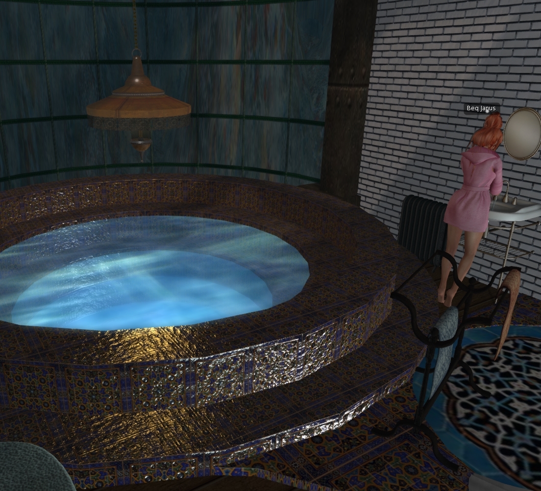
It is time to do a little more work on a slow burn project to gradually rebuild parts of my ancient underwater home. I've only got half an hour to spare so I want to Mesh the steps in the moonpool, so that I can safely apply some materials without it blowing up.


I quickly copy the existing object, tossed in the joined mesh script, eliminate a couple of the unnecessary surfaces and hit "Mesh".


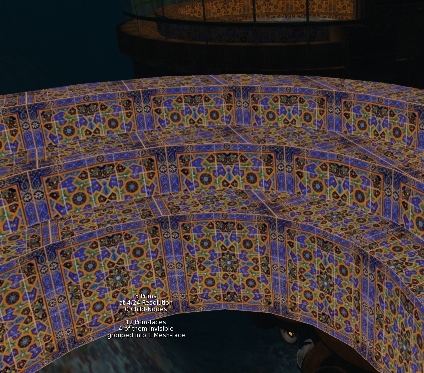
A few moments later and I have it imported, apart from being a few Lindens poorer, we are good to go,aren't we? I drag the texture onto the Mesh and....ugh! That was a waste a Lindens, the texture UV mapping is wrong.

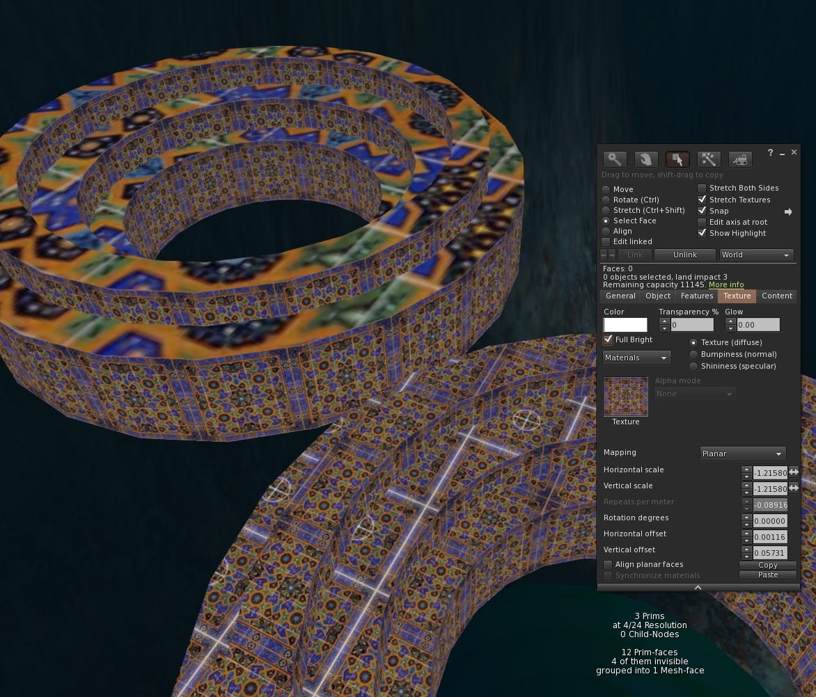
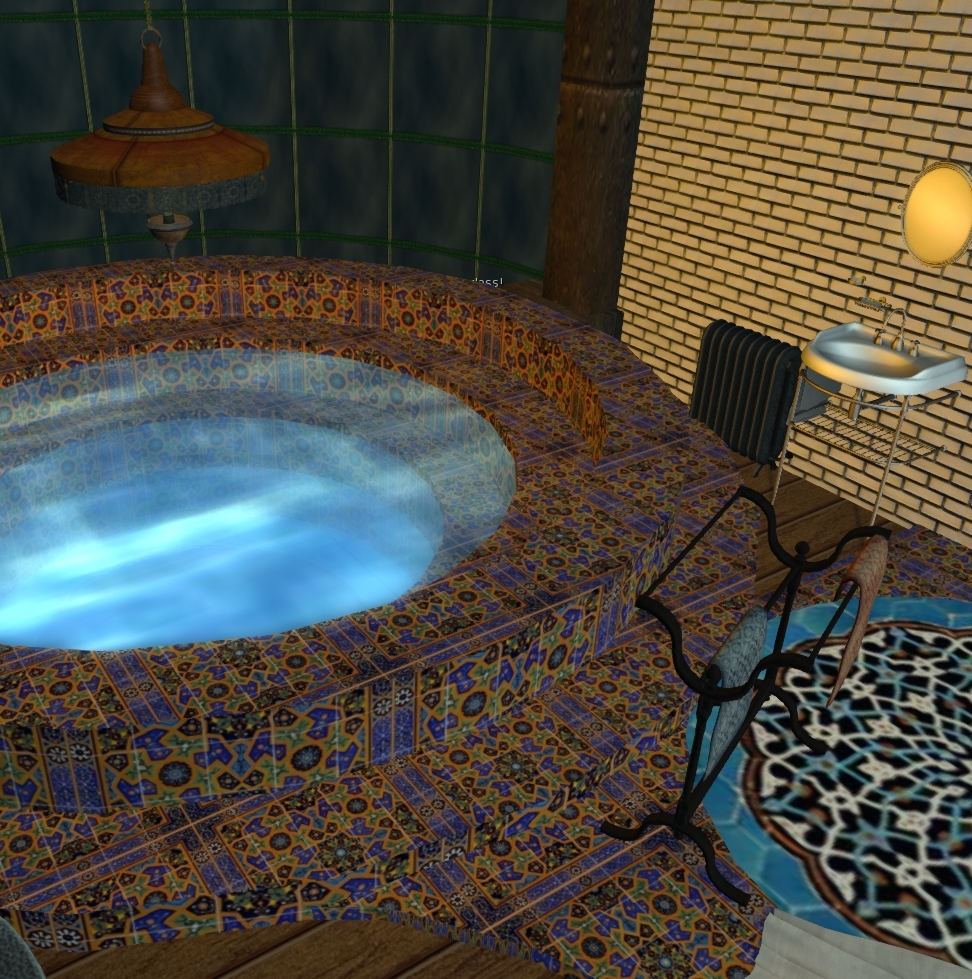
 A quick check of the source model and the reason is clear. While MS quite correctly noted that the texture UUID and the tint are the same on all the faces, it failed to note that top faces were planar mapped, while the inside cylinder faces were default mapped.


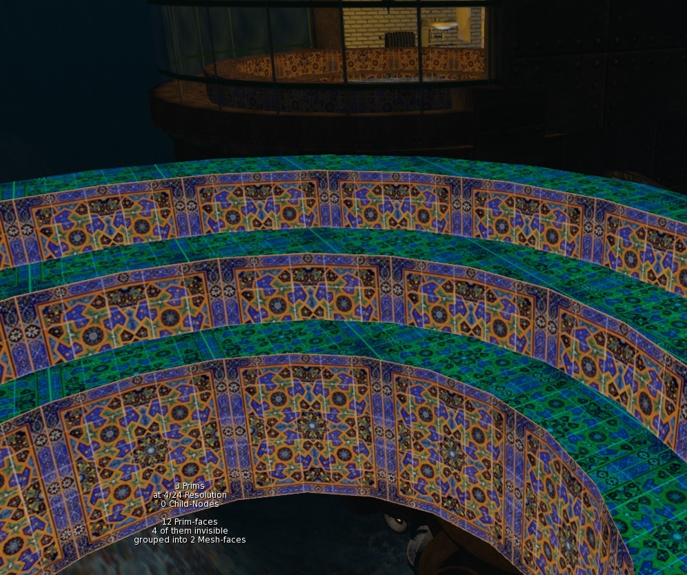
Happily, this is easily fixed. All we need to do is convince MS that this is a different face to the other one. We can do that by changing the tint value. A quick lick of paint and we find that MS now correctly sees this as having two mesh faces. and we are ready to splash another few lindens on an upload.


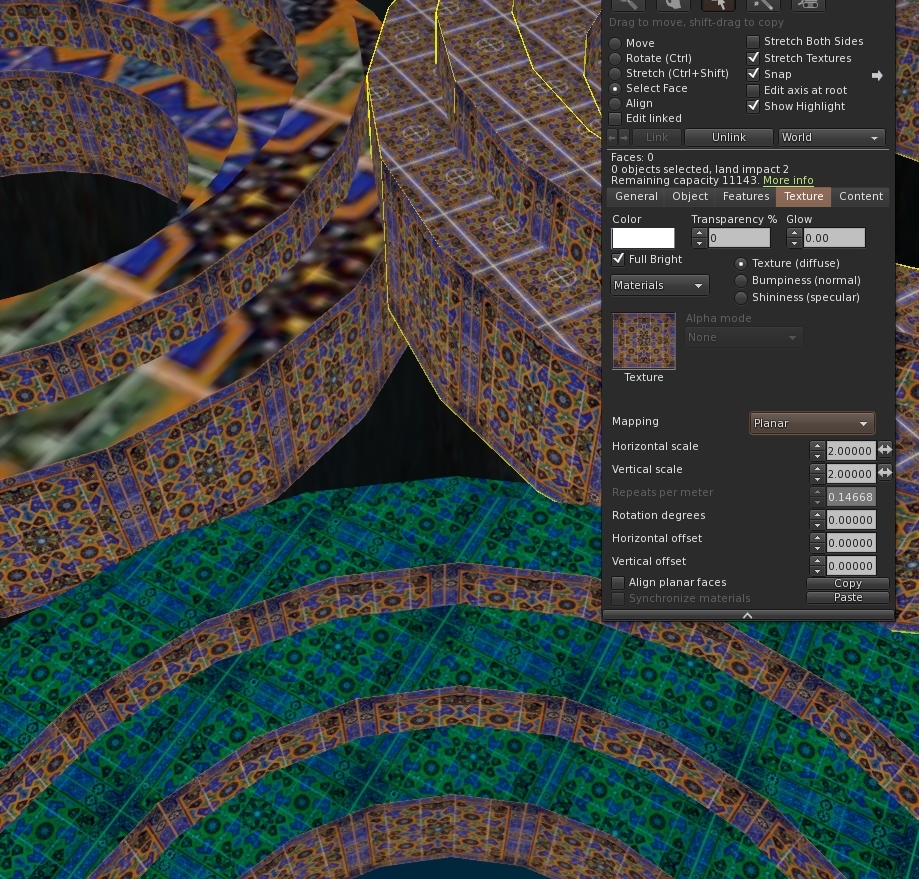
Rezzing the newly uploaded mesh we gleefully drop out texture on it and for a moment our hearts skip a beat. It still looks the same. Then we remember, it's called "default" mapping for a reason and sure enough highlighting the face and setting the mapping mode to planar snaps it back into shape.


And so there we have it. When mixing planar and non-planar with the same texture just make sure that they have a different tint.

If you have a larger build that will be painful to convert manually I have written a script that runs through the material list, identifies clashes and auto-magically changes the tint. Ping me an IM inworld and I'll send you a copy until I get around to putting it up to download somewhere.

I'm heading out for a couple of weeks so take care and more blogs when I return.
For now, I'll close with a quick recap of the steps with some materials applied to give the tiles that glazed shine.A bit overdone but mission accomplished for the Mesh at least.

Love

Beq
x


Saturday, 30 July 2016

Blender mesh data deep dive.

It's been a while since we last had a post on my quest to write better workflow tools for Second Life Mesh creators using Blender. In the last of that series, we took a long hard look at what exactly was meant by download cost and why our naive triangle counter was giving us such overestimates. Now it is time to try to use some of that knowledge to see how we can build that from Blender.

Decompression sickness

It was the compressed byte stream that was throwing out our numbers and, as a result, we will need to reproduce the data and compress it to find the byte streaming cost. This means that we need to look at how the polygons are stored in Blender.

We did a little of this when we were counting the triangles but we barely scratched the surface. 
All the data we need is in the bpy.data structure for a mesh object.

The BPY data structure is not very well documented but there is a lot of code around and the excellent blender python console that lets you try things out and features autocomplete.

Given an arbitrary mesh object (obj) we can access the mesh data itself through obj.data

import bpy

obj = bpy.context.scene.objects.active # active object

mesh = obj.data
Within obj.data we have access to a list of vertices and a list of polygons and a vast array of other attribute and views on the data.

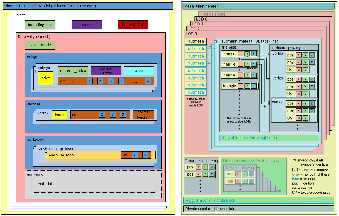
Following in the footsteps of the wonderful visualisation of the SL Mesh Asset Format by Drongle McMahon that we discussed in a previous blog I have had a stab at a comparable illustration that outlines the parts of the blender bpy data structure that we will need access for our purposes
On the left, we have my "good parts version" of the BPT datastructure, while on the right we have the SL Mesh Asset visualisation from Drongle McMahon's work.

We can now start to list out the differences and thus the transformations that we will need to apply
  1. SL Mesh holds all the LODs in one "object". We have multiple objects, one per LOD.
  2. A Mesh object has a list of polys that index into a list of vertices. SL has multiple meshes, split as one per material face
  3. SL only accepts triangle, we have Quads and NGons as well.
  4. Each submesh is self contained, with triangles, UVs, normals and vertices listed. Vertices are thus duplicated where they are common to multiple materials.
  5. SL data is compressed
So let's sketch out the minimum code we are going to need here.

For each Model in a LOD model set.
    Iterate through the polygons, and separating by material
    For each resulting material mesh
        for each poly in the mat mesh
             add new verts to the vert array for that mat. mesh
             adjust the poly into triangles where necessary
             add the resulting tris to the material tri array
             write the normal vector for the triangles
             write the corresponding UV data.
    compress the block

Having done the above we should be able to give a more accurate estimate.

A lot easier said than done...Time to get coding...I may be some time.

Love

Beq
x


Saturday, 16 July 2016

When is a triangle not a triangle? (mesh streaming)

When is a triangle not a triangle?
(when it's compressed)

Welcome to this 6th in the series of blog posts examining the task of creating a Blender Addon to assist with our Second Life Mesh creation workflows.

In the last post, we discovered that all was not quite as it seems in the mesh streaming calculation. Our carefully recreated algorithm repeats all the steps that the published documentation discusses and yet the results did not match. We further learned that this was most likely down to the "estimation" process.

So what is the problem here?

The clue is in the name, "Mesh Streaming Cost" it is intended to "charge" based on the cost of streaming the model; so what does that mean? In real terms it means that they are not looking at the difficulty of rendering an object directly, they are looking at the amount of data that has to be sent across the network and processed by the client. When we export models for use in Second Life we typically use Collada format. Collada is a sprawling storage format that uses a textual XML representation of the data it is very poorly suited to streaming across the internet. This problem is addressed by the use of an internal format better suited to streaming and to the way that a virtual world like Second Life works.

What does the internal format look like?

We can take a look at another of the "hidden in plain sight" wiki pages for some guidance.
The Mesh Asset Format page is a little old, having last been updated in 2013 but it should not have fundamentally changed since then. Additions to SL such as normal and specular maps are not implemented as part of the mesh asset and thus have no effect. It may need a revision in parts once Bento is released.

The page (as with many of the wiki pages nowadays) has broken image links. There is a very useful diagram by Drongle McMahon that tells us a lot about the Mesh Asset Format in visual terms.


In my analysis of the mesh streaming format, it became clear that while Drongle's visualisation is extremely useful it lacks implementation specific details. In order to address this, I looked at both the client source code but also the generated SLM data file for a sample mesh and ended up writing a decoder based upon some of the older tools in the existing viewer source code.
{ 'instance': 
   [ # An array of mesh units
    { 'label': 'Child_0', # The name of the object
                  'material': 
       [  # An array of material definitions
        { 'binding': 'equatorialringside-material',
                     'diffuse': { 'color': [ 0.6399999856948853,
                                             0.6399999856948853,
                                             0.6399999856948853,
                                             1.0],
                                  'filename': '',
                                  'label': ''},
                     'fullbright': False
        }
       ]
       'mesh_id': 0, # A mesh ID, this is effectively the link_id of the resulting linkset
       'transform': [ 10.5, 0.0, 0.0, 0.0,
                      0.0, 10.455207824707031, 0.0, 0.0,
                      0.0, 0.0, 5.228701114654541, 0.0,
                      0.0, 0.0, 2.3643505573272705, 1.0]
    }
   ],
  'mesh': 
   [ # An array of mesh definitions (one per mesh_id)
    { # A definition block
     'high_lod': {'offset': 6071, 'size': 21301},
     'low_lod': {'offset': 2106, 'size': 1833},
     'lowest_lod': {'offset': 273, 'size': 1833},
     'material_list': 
         [ # array of materials used 
          'equatorialringside-material',
          'equatorialringsurface-material',
          'glassinner-material',
          'glassouter-material',
          'strutsinnersides-material',
          'strutsinnersurface-material',
          'strutsoutersides-material',
          'strutsoutersurface-material'
         ],
     'medium_lod': {'offset': 3939, 'size': 2132},
     'physics_convex': {'offset': 0, 'size': 273}
     <compressed data=""> 
     # LENGTH=SUM of all the size parameters in the LOD and Physics blocks
    }
   ],
  'name': 'Observatory Dome', # name of the given link set
  'version': 3  # translates to V0.003
}

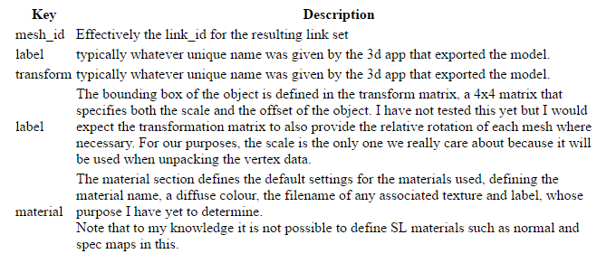
All of this is an LLSD, a Linden Lab structure used throughout the SL protocol,  effectively an associative array or map of data items that is typically serialised as XML or binary. The header portion contains version information, and an asset name, it can also have the creators UUID and the upload date (if it came from the server) .

We also see two other top level markers, 'instance' and 'mesh', this is the stuff we really care about.

Instance

'Instance' is an array of mesh units that form part of the link set. Often when people work with mesh they use a single mesh unit but you can upload multipart constructs that appear inworld as a link set.
Each instance structure contains a set of further definitions.


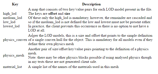
Mesh

The final entry in the header is the mesh array. Like the instance array before it the mesh array has one entry for each mesh unit and as far as I am able to tell it must be in Mesh_id order.
The mesh structure in the array is another LLSD with the following fields:-


At the end of each Mesh is the compressed data that is represented by the bulk of Drongle's diagram and it is for this that we have been waiting for this is why our naive triangle counting solution is giving us the wrong answer.

Compressed mesh data

At the end of each Mesh block is an area of compressed data. Space for this is allocated by the SLM "mesh" entry whose length includes the compressed data even though it is not strictly part of the LLSD.

Once again we need to look at both Drongle's excellent roadmap and the viewer source code to work out precisely what is going on.

As you will recall the Mesh section defined a series of size and offset values, one pair per stored model. In my examples, the physics_convex is always the first model and thus has offset 0.

physics_convex

{ 'BoundingVerts': 'ÿÿÿ\x7f\x00\x00\x81Ú\x81Úa\x18þ\x7fæyþÿÿ\x7f\x00\x00\x
8}%\x81Úa\x18\x00\x00ÿ\x7fa\x18}%}%a\x18ÿ\x7fÿÿa\x181Ö\x16\x86\x97¸Ì)\x17\
                   '¯nÈ\x97¸\x00\x00ÿ\x7f\x00\x00\x9eO\x9aÇ\x94¸Äµ\x92í2\x
                   ':Jl\x12.\x0c'
                   '«·a\x133\x0c'
                   'SH\x9dì.\x0c'
                   'T\x85'
                   '\t}þÿªzò\x82þÿF\x85'
                   '\r'
                   '\x83þÿ¸zô|þÿ',
  'Max': [0.5, 0.5, 0.5],
  'Min': [-0.5, -0.5, -0.5]}

Here we see that the compressed data is really just another LLSD map. In this case, we have three keys, Max, Min and BoundingVerts.

Max and Min are important, we will see them time and again and in most cases, they will always be 0.5 an -0.5 respectively. These define the domain of the normalised coordinate space of the mesh. I'll explain what that means in a moment.

BoundingVerts is binary data. We will need to find another way to show this and then to start to unpick it.

['physics_convex']['BoundingVerts'] as hex
dumping 18 bytes:
00000000: FF FF 00 00 00 00 00 00  00 00 FF FF 00 00 FF FF  ................
00000010: 00 00                                             ..

This is the definition of the convex hull vertices, but it has been encoded. Each vertex is made of three coordinates. The coordinates have been scaled to a 1x1 cube and encoded as an unsigned short integer. Weirdly the code to do this is littered throughout the viewer source, where a simple inline function would be far more maintainable. But we're not here to clean the viewer code.
In llmodel.cpp we find the following example

 //convert to 16-bit normalized across domain
 U16 val = (U16) (((src[k]-min.mV[k])/range.mV[k])*65535);

In python, we can recreate this as follows.

def ushort_to_float_domain(input_ushort, float_lower, float_upper):
    range = float_upper - float_lower
    value = input_ushort / float(65535) # give us a floating point fraction 
    value *= range # target range * the fraction gives us the magnitude of the new value in the domain
    value += float_lower # then we add the lower range to offset it from 0 base
    return float(value)

There is an implication to this of course. It means that regardless of how you model things your vertices will be constrained to a 64k grid in each dimension. In practice, you are unlikely to have any issues because of it. And so applying this knowledge we can now examine the vertex data.
expanding using LittleEndian
0: (65535,0,0)->(0.500000,-0.500000,-0.500000)
1: (0,0,65535)->(-0.500000,-0.500000,0.500000)
2: (0,65535,0)->(-0.500000,0.500000,-0.500000)
Max coord: 65535 Min coord: 0

It is my belief that these are little-endian encoded. The code seems to support this but we may find that we have to switch that later.

We can apply this knowledge to all sets of vertices.

Onwards into the Mesh

Looking into the compressed data we find that the LOD models now follow. They follow in the order that you'd expect, lowest to high.

Each LOD model represents the actual vertex data of the mesh. Mesh data is stored as a mesh per material, thus we find the compressed data section per LOD is comprised of an array /list of structures or what Drongle refers to as a submesh in his illustration, one element of the array for each material face. Each material face is the comprised of a structure of the following:
Field
Description
Normal
A list of vector normal that corresponds to the vertices
Position
The vector cords of the vertices
PositionDomain
The min and max values for the expanded coord data (as per the preceding physics section)
TexCoord0
The UVW mapping data. At present, I have not investigated the encoding of this, but it would appear to be the case that these are encoded identically to the Vertex data but with only the X and Y components.
TexCoord0Domain
The min/max domain values associated with the UVW data
TriangleList
The mesh, a list of indices into the other data fields (the Position, TexCoord and Normal) that form the triangles of the mesh itself. Each triangle in the lost is represented by three indices, which refer uniquely to an entry in the other tables.Individual indices may of cours be shared by more than one triangle.

I think this is more than enough for one post. We've covered a lot of ground.
I am now able to successfully decode an SLM asset in Python and so next we can see how this helps us calculate the LI.

love Beq
x

Thursday, 7 July 2016

The truth about mesh streaming

The truth about mesh streaming

Ever wondered why a mesh with the same number of triangles could give different LI? Or how the impact of each LOD model is assessed? Stick with me today and hopefully, I'll show you.

Today's post is the fifth in the series of meanderings through Blender Addons. Yesterday, we left things in an OK state. My AddOn is reflecting the correct triangle counts for the models (and correctly associating the models with the LOD they represent).

Today we will look at the Mesh Streaming Cost algorithm and have a go at converting that to python.
This is an unashamedly technical blog. I will try to explain some aspects as I go through but the nature of the topic demands some technical detail, quite a lot of it.

I am going to work from the latest Firestorm Viewer source, and a couple of somewhat outdated wiki resources. The wiki resources themselves should be good enough, but the problem with them is that you can never be sure if things have been tweaked since. Ultimately though we have a real world comparison, our estimates should match (or be close to) the Viewer upload, we will test this at the very end.

A good place to start is the Mesh Streaming Cost wiki page as with many wiki documents it is out of date and not entirely correct. However, we can use it as a starting place. The concept section explains the thought behind this. The equation part is where we will start.
  1. Compute the distance at which each LOD is displayed
  2. Compute the area in which each LOD is relevant
  3. Adjust for missiing LODs
  4. Scale relative weights of each LOD based on what percentage of the region each LOD covers.
  5. Compute cost based on relevant range and bytes in LOD
It goes on to tell us what the LOD transition distances are, details we covered in the post yesterday.

Using these we can write another helper function
def getLODRadii(object):
    max_distance = 512.0
    radius = get_radius_of_object(object)
    dlowest = min(radius / 0.03, max_distance)
    dlow = min(radius / 0.06, max_distance)
    dmid = min(radius / 0.24, max_distance)
    return (radius, dmid, dlow, dlowest)

This function takes an object and using our previously written radius function and applying the knowledge above, returns a list of values. The radius itself, the High to Mid transition distance, The Mid to low transition and finally the Low to Lowest.

We use a constant max distance of 512 as it matches that used in the code example and the current live code. Quite why it should be 512 (2 regions) is unclear to me.

So now we should be able to add a new column to our display and show the LOD change radii

Step 2 is to compute the area for each LOD. Now that we have the Radius that is a simple task.

def area_of_circle(r):
    return math.pi * r * r

The function above returns the area for a given radius.

The next step is "Adjusting for missing LODs", we'll take this into account when we display things. But in terms of the algorithm, if a given LOD is missing then the next highest available LOD is used.

We can now progress to the "Computing Cost" section. This section gives use the following formula.

    Streaming Cost =
        (   (lowest_area / total_area) * bytes_in_lowest
          + (low_area    / total_area) * bytes_in_low
          + (mid_area    / total_area) * bytes_in_mid
          + (high_area   / total_area) * bytes_in_high   ) * cost_scalar
The first part is a ratio, a weighting applied to the LOD based upon the visibility radii.
The second part is more confusing on its own, "bytes_in_LOD" where did that come from?

The answer lies in the note just below the pseudo code.
In the details of the implementation, the cost_scalar is based on a target triangle budget, and efforts are made to convert bytes_in_foo to an estimated triangle count.
So what does that mean exactly? The answer lies in the C++ code below it and, in particular:
F32 bytes_per_triangle = (F32) gSavedSettings.getU32("MeshBytesPerTriangle");
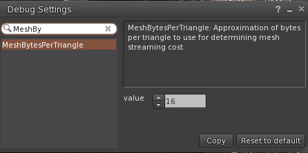
This is a setting stored in the viewer that approximates how many bytes are in a triangle for the purpose of converting "bytes" to triangles. Looking at the current live viewers, we find that the setting has a value of 16.

This value is then used to convert a bytes_LOD value to a triangles_LOD value.
    F32 triangles_high   = llmax((F32) bytes_high-METADATA_DISCOUNT, MINIMUM_SIZE
                            /bytes_per_triangle;
This deducts a METADATA_DISCOUNT constant to remove the "overhead" in each mesh LOD to leave only the real triangle data. The remaining bytes are divided by our bytes_per_triangle to get the number of triangles. This raises the question of whether 16 is the right "estimate" Indeed, why is it an estimate at all? In Blender we won't be estimating, we know how many triangles we have. However, it will turn out that the page is missing one vital piece of information that explains all of this...However, we will come back to this once we have worked out the rest.

Looking in more detail at the implementation we find that lowest area and the related "areas" are not quite what they seem.
In the C++ implementation, we observe that high_area is indeed the area of the circle defined by the roll off point from High to Medium LOD,
F32 high_area   = llmin(F_PI*dmid*dmid, max_area);
but we discover that mid_area is the area of the medium range only, excluding the high_area. The area of the Ring in which the Medium LOD is visible.The same applies to the others.

Putting this all together in python we get the following:-

def getWeights(object):
    (radius, LODSwitchMed, LODSwitchLow, LODSwitchLowest) = getLODRadii(object)

    MaxArea = bpy.context.scene.sl_lod.MaxArea
    MinArea = bpy.context.scene.sl_lod.MinArea

    highArea = clamp(area_of_circle(LODSwitchMed), MinArea, MaxArea)
    midArea = clamp(area_of_circle(LODSwitchLow), MinArea, MaxArea)
    lowArea = clamp(area_of_circle(LODSwitchLowest), MinArea, MaxArea)
    lowestArea = MaxArea

    lowestArea -= lowArea
    lowArea -= midArea
    midArea -= highArea

    highArea = clamp(highArea, MinArea, MaxArea)
    midArea = clamp(midArea, MinArea, MaxArea)
    lowArea = clamp(lowArea, MinArea, MaxArea)
    lowestArea = clamp(lowestArea, MinArea, MaxArea)

    totalArea = highArea + midArea + lowArea + lowestArea

    highAreaRatio = highArea / totalArea
    midAreaRatio = midArea / totalArea
    lowAreaRatio = lowArea / totalArea
    lowestAreaRatio = lowestArea / totalArea
    return (highAreaRatio, midAreaRatio, lowAreaRatio, lowestAreaRatio)

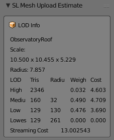
This should give us the weighting of each LOD in the current models at the current scale. So let's add this to our display.

Here we can see that our Medium and Low LODs are carrying a lot of the LI impact and thus if we want to manage the LI we need to pay a lot of attention to these. The more observant will note that the Lowest is effectively 0, and yet we are telling it to use the LOD from the LOW, this makes no sense at first glance, it should be very expensive. The explanation is in the radius column. Lowest does not become active until 261m, which is outside of the 256m maximum  (see maxArea in the code above), this means that the Lowest is clamped to a radius of 256, which matches the radius of the Low and thus results in 0 weight.

With all this in place, we are finally able to have a first run at calculating the streaming cost.
Once again we refer to the C++ implementation for guidance.
    F32 weighted_avg = triangles_high*high_area +
                       triangles_mid*mid_area +
                       triangles_low*low_area +
                       triangles_lowest*lowest_area;
 
    return weighted_avg/gSavedSettings.getU32("MeshTriangleBudget")*15000.f;
 In our python translation this becomes:

        weightedAverage =   hi_tris*highAreaRatio + mid_tris*midAreaRatio + low_tris*lowAreaRatio + lowest_tris*lowestAreaRatio
        streamingCost = weightedAverage/context.scene.sl_lod.MeshTriangleBudget*15000

I am not a fan of the magic numbers used here (MeshTriangleBudget is in fact another viewer setting and has a value of 250000, the 15000 however is a simple hard coded constant so we have little choice but to replicate it.

For our final reveal for tonight then let's see how out LI calculation has performed.


Oh dear...
Well, I guess it had all been too easy so far.
The Firestorm upload has calculated that this object will have a streaming impact of 8LI
Our determination has calculated 13LI. That is a considerable difference, what could possibly have gone wrong?

The answer was hinted at previously; it is to do with the estimate, the bytes_LOD values and what they actually are. The problem lies in the fact that your mesh is not sent back and forth unaltered from the DaE file that you upload. In fact, it is uploaded in an internal format that compresses each LOD model. The bytes_LOD values represent the compressed size of the actual mesh that will be streamed, the estimated bytes_per_triangle of 16 is, it would seem greatly underestimating the compression level.
In my next blog, I will examine the internal format in more detail. We'll explain why the estimated bytes per triangle is wrong, and we will start to work out how we can make this work.

Until then, thank you for reading this blog. Please share or +1 if you have found it useful, or if you think that your friends might.

Love
Beq
x

Wednesday, 6 July 2016

Mesh accounting mayhem

Mesh accounting - Download/streaming costs

This post is the 4th in this series of posts about Blender Addons for SecondLife creation, and we (finally) get to sink our pythonic fangs into something concrete.

Previously...

Post 1 - We started to put a simple addon together to generate five copies of a selected Mesh and rename them according to their intended use.
Post 2 - We took it a step further by allowing the user to select which LOD to use as the source and which targets to produce.
Post 3 - We wrapped up the process, connecting the execute method of the operator to the new structures maintained from the UI.

So what next?

Tonight we are going to try (or at least start) to replicate the streaming cost calculation of SL in Blender.

A quick recap

For those who have not looked lately and are perhaps a little rusty on Mesh accounting here is the summary.
Firstly, I will use the term Mesh primitive to denote a single mesh object that cannot be decomposed (unlinked) in-world. It is possible to link Mesh Primitives together and to upload a multi-part mesh exported as multiple objects from a tool such as Blender.

The LI (Land Impact) of a Mesh primitive is defined as being the greater of three individual weights.
1) The streaming or download cost
2) The Physics cost
3) The server/script cost

Mathematically speaking if D is Download, P is physics and S is streaming then
LI = round(max(D,P,S)) 
Of these S is simplest and generally speaking least significant. It represented the server side load, things like script usage and essential resources on the server. At the time of upload, this is 0.5 for any given Mesh primitive; this means that the very lowest LI that a Mesh primitive can have is 0.5, and this rounds up to 1 in-world. Because the rounding is calculated for the entire link set,  two Mesh primitives of 0.5 each, can be linked to one another and still be 1LI (in fact three can because 1.5LI gets rounded down!).
Physics cost we will leave to another post,  much misunderstood and often misrepresented, it is an area for future discussion.
And so that leaves Streaming cost,
If you read my PrimPerfect (also here) articles on Mesh building in the past, you will know that the streaming cost is driven by the number of triangles in each LOD and the scale of the object.
LOD, or Level Of Detail, is the term used to describe the use of multiple different models to deal with close up viewing and far away viewing. The idea being that someone looking in your direction from half a region away does not want to download the enormous mesh definition of your beautifully detailed silver cutlery. Instead, objects decay with distance from the viewer. A small item such as a knife or fork will decay to nothing quite quickly, while a larger object such as a building can reasonably be expected to be seen from across the sim. Even with a large building,  the detailing of the windows, that lovely carving on the stone lintel on the front door, and so forth, are not going to be discernable so why pay the cost for them when a simpler model could be used instead? Taking both of these ideas together it is hopefully clear why scale and complexity are both significant factors in the LI calculation.


The highest LOD model is only visible from relatively close up. The Medium LOD from further away, then the low and the lowest. Because the lowest LOD can be seen from anywhere and everywhere the cost of every triangle in it is very high. If you want a highly detailed crystal vase that will be "seen" from the other side of the sim, then you can do so, but you will pay an extremely high price for it.

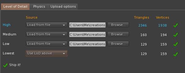
The way that most of us see the streaming cost is through the upload dialogue. Each LOD model can be loaded or generated from the next higher level. One rule is that each lower LOD level must have the same or fewer triangles than the level above it.

When I am working in Blender, I export my Mesh files, drop into the upload dialogue and see what it would cost me in LI. I then go back and tweak things, etc, etc. Far from the ideal workflow.

One of my primary goals in starting this process was to be able to replicate that stage in Blender itself. It can't be that hard now, can it?

..Sadly, nothing is ever quite as easy as it seems, as we will find out.

To get us started, we need to get a few helper functions in place to get the Blender equivalent functions.

We will need to know the dimensions of the object and the triangle count of each LOD Model.
This is why we wanted a simple way to link models that are related so that we can now do calculations across the set.


def get_radius_of_object(object):
    bb = object.bound_box
    return (Vector(bb[6]) - Vector(bb[0])).length / 2.0

The function above is simple enough, I do not like the magic numbers (0 and 6) and if there is a more semantic way to describe them I would love to hear of it, but they represent two extreme corners of the bounding box and the vector between them is therefore 2* the radius of a sphere that would encompass the object.

def GetTrianglesSingleObject(object):
    mesh = object.data
    tri_count = 0
    for poly in mesh.polygons:
        tris_from_poly = len(poly.vertices) - 2
        if tris_from_poly > 0:
            tri_count += tris_from_poly
    return tri_count

The function here can (as the name suggests) be used to count the triangles in any object,
At first thought, you might think that, with triangles being the base of much modelling, there would be a simple method call that returned the number of triangles, alas no. In Blender, we have triangles, and quads and ngons, A mesh is not normally reduced to triangles until the late stages of modelling (if at all) to maintain edge flow and improve the editing experience. Digital Tutor have an excellent article on why Quads are preferred.

The definitive way to do this is to convert a copy of the mesh into triangles using Blenders triangulate function, but we want this to work in realtime, and the overhead of doing this would be phenomenal. The method I settled on was a mathematical one. The Mesh data structure in Blender maintains a list of polygons. Each Polygon, in turn, has a list of vertices. We can, therefore, iterate over the polygon list and count the number of vertices in each poly. For each polygon, we need to determine the number of triangles it will decompose in to. A three-sided is a single triangle, of course, A four-sided polygon, a quad, decomposes, ideally, into two triangles, a five-sided poly gives us a minimum of three. The pattern is clear. For a polygon with N sides, the optimal number of triangles is N-2. What is less clear to me is whether there are cases that I am ignoring here. There are many types of mesh some more complex than others. If there are cases where certain types of geometry produce no conformant polygons, then this function will not get the correct answer. For now, however, we will be content with it and see how it compares to the Second Life uploader's count.

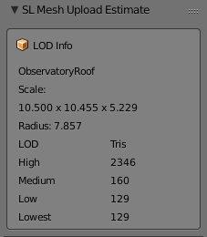
Armed with these helper functions, and the work we did previously, we can now add the counts that we need to a new Blender UI panel as follows.

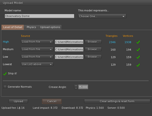
So let's see if this compares well with the Second Life Mesh uploader.

Spot on. So far so good. Enough for one night, tomorrow we'll take a deeper dive into the streaming cost calculation.

Beq
x
Tuesday, 5 July 2016

Snake charming in Blender part 3 -

This blog post is the third in the series of posts on my Blender AddOn adventures.

Previously:-
Post 1 - We started to put a simple addon together to generate five copies of a selected Mesh and rename them according to their intended use.
Post 2 - We took it a step further by allowing the user to select which LOD to use as the source and which targets to produce.

At the end of the last post we had the user interface elements working but they had not be wired up to the addon itself.

The code for this blog has taken a while for me to get to the point where I am properly happy with it as it required a bit more background reading to make the work covered in the last blog initialise itself correctly. This blog post, however, should be quite short and then we will move on to something more interesting.

In the first, naive, version we had a simple function that created 5 duplicate copies of a base object. There are lots of different workflows that can be followed and, for me at least, it varies a little depending on what I am building, where I am starting from etc.  I work on a Mesh I often end up working in two directions. I upload a template made using Mesh Studio in SL, this gives me a proforma with the right scale and a little confidence that it will fit where it needs to. That template can often evolve into the medium LOD, then get duplicated, adding detail and refinement to use as the high LOD model and then removing things from another copy to form the low LOD.

It was also a good chance to refactor the repetitive code from the first version.

The execute method of the operator is now far more generic. I have created support functions for stripping the LOD extension from an object name. This means that I can quickly get from any LOD model to any other by removing the extension and adding another, the upshot of this is that you do not need to be looking at the HIGH LOD model in order to generate another clone from it.

def execute(self, context):
# For every selected object
        for object in context.selected_objects:        
            basename = self.getSLBaseName(object.name)  
# strip the _LOD if any to find the "root" name
            source = self.findOrCreateSourceModel(basename, context)
# locate the source LOD Model if it exists, if not create it using the selected mesh
            if(source is not None):
                for i in context.scene.sl_lod.LOD_model_target:
                    # For every target LOD clone the src and relocate it to the correct layer
                    targetModel=self.createNewLODModel(source, self.getLODAsString(i))
                    self.moveToLayers(targetModel, {int(i)})                    
        return {"FINISHED"}

That's all for this blog, it was wrapping up a few loose ends, though the brevity of the blog does not reflect the pain of learning how to get properties to register properly in Blender.


Monday, 13 June 2016

Adventures in Blender scripting - automating workflow

Blender Addons

I have decided to have a go at writing a Blender Addon to ease my Second Life Mesh development workflow.

I will approach this in a modular manner hoping to learn a lot about both Python and Blender as I go.

When I build in Blender I tend to either start with a Mesh Studio model and perhaps generate a series of LODs using that tool or create a High LOD model and duplicate it for the lower LODs. Having duplicated them I can then set about reducing the complexity.

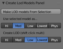
The first task is to create a simple operator to take a selected objects and create duplicates that will be used as the Medium, Low, Lowest and perhaps even Physics meshes.